Chemical Engineering
From questions to insights, 30online scientific tool. No registration required, free calculation and export.
Distillation Designer
uses operating lines and plate-by-plate ladders to understand separation and reflux ratios.
Binary constant relative volatility, constant molar flow; the equilibrium stage includes a partial reboiler and does not include a total condenser. Unreachable separation and pinch return diagnostics.

Unit Operations
solves two-phase flash evaporation for a given K value, or calculates the heat exchanger outlet state.
flash evaporation uses the input constant K and does not automatically call the physical property library; the heat exchanger is a counterflow ε–NTU model with constant heat capacity.
Recycle Flowsheet
solves the steady-state process consisting of mixing, reaction, separation and reflux.
fixed topology: fresh feed→mixing→A converted into B→B complete separation→A split and reused; supports parameters of each unit, non-universal process simulator.

Reynolds Number
Calculates pipe flow Reynolds number and demonstrates velocity sensitivity.
circular tube flow regime threshold is only an empirical reference, and disturbances and inlet conditions will change the transition.
Darcy–Weisbach Pressure Drop
calculates the pressure drop and Darcy friction factor along the circular pipe.
Laminar flow f=64/Re; turbulent Haaland approximation; transition zone rejected; no local losses included.
Log Mean Temperature Difference
estimates LMTD and heat transfer based on the temperature at the four ends of the counterflow.
Steady counterflow, constant U; does not include complex flow pattern correction coefficients.
First-order CSTR
calculates the ideal stirred tank residence time and volume based on the target conversion rate.
Steady-state, isothermal, constant density, irreversible first-order reaction.
First-order PFR
Calculate the residence time and volume of an ideal plug flow reactor.
Isothermal, constant density, irreversible first-order reaction.
Water Vapor Pressure
Calculates the saturated vapor pressure of liquid water at 1–100 °C.
limits the empirical temperature zone below the normal pressure boiling point of water, and the output pressure is converted from mmHg to kPa.

Ideal Gas State
calculates the volume and density of ideal gases and displays isothermal compression curves.
is a rarefied ideal gas with a temperature of K; high pressure or near saturation requires a real gas model.

Binary Stream Mixing
w=(m₁w₁+m₂w₂)/(m₁+m₂): Calculate the mass fraction mixing of two streams according to the input, and provide local sensitivity curves and data export.
Steady-state mixing process with no reaction and no loss of components.
Sensible Heat Duty
Q=ṁcpΔT: Calculate sensible heat load based on input, provide local sensitivity curve and data export.
has constant specific heat, no phase change, and no chemical reaction.
Latent Heat Duty
Q=ṁΔh: Calculate the phase change latent heat load based on the input, and provide local sensitivity curves and data export.
The input enthalpy difference needs to match the pressure and material.
Heat Transfer Area
A=Q/(UΔTlm): Preliminary calculation of heat transfer area based on input, providing local sensitivity curve and data export.
The ideal counterflow correction coefficient is one; the actual design requires dirt and structural corrections.

Heat Exchanger NTU
NTU=UA/Cmin: Calculate heat exchanger NTU based on input, provide local sensitivity curve and data export.
Definition of the number of heat transfer units for the ε–NTU method.
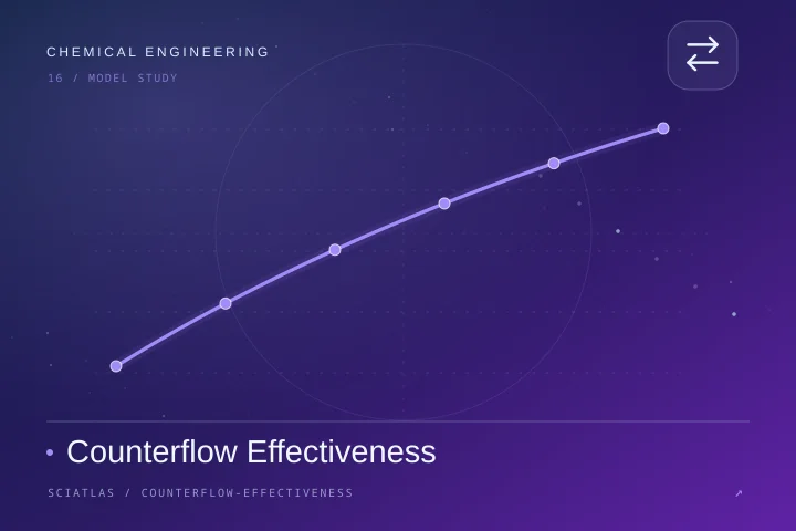
Counterflow Effectiveness
ε=[1−exp(−NTU(1−Cr))]/[1−Cr exp(−NTU(1−Cr))]: Calculate the effectiveness of the counterflow heat exchanger based on the input, and provide local sensitivity curves and data export.
Ideal countercurrent, constant physical properties, no heat loss; Cr=1 uses the continuous limit.

Prandtl Number
Pr=cp μ/k: Calculate Prandtl number based on input, provide local sensitivity curve and data export.
Thermal momentum diffusivity ratio, all physical properties must be taken at the same temperature.

Schmidt Number
Sc=μ/(ρD): Calculate the Schmidt number based on the input, and provide local sensitivity curves and data export.
Ratio of momentum to mass diffusivity.

Peclet Number
Pe=vL/α: Calculate the Peclet number based on the input, and provide local sensitivity curves and data export.
can be used for heat or mass transport, and the physical meaning of the diffusivity used must be clarified.
Hagen Poiseuille Pressure Drop
ΔP=128μLQ/(πd⁴): Calculate the laminar flow circular tube pressure drop based on the input, and provide local sensitivity curves and data export.
Fully developed Newtonian laminar flow circular tube; check Re<2300, excluding inlet and local losses.
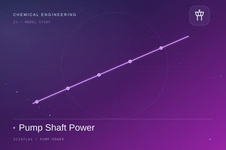
Pump Shaft Power
P=ρgQH/η: Calculate the pump shaft power based on the input, and provide local sensitivity curves and data export.
Incompressible fluid; motor losses must be calculated separately.
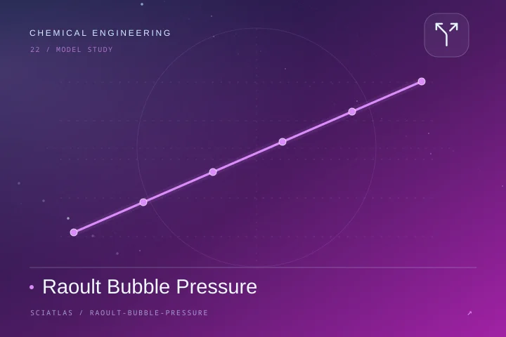
Raoult Bubble Pressure
P=x₁P₁sat+(1−x₁)P₂sat: Calculate the ideal binary bubble point pressure based on the input, and provide local sensitivity curves and data export.
The ideal liquid phase and the ideal gas phase are at the same temperature and have no azeotropic behavior.
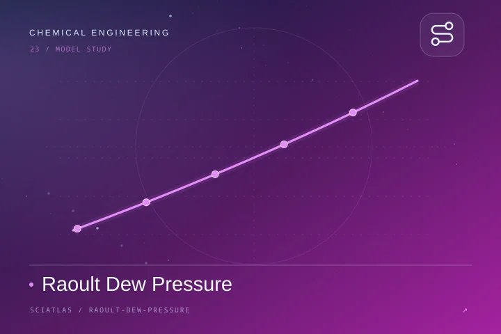
Raoult Dew Pressure
P=1/[y₁/P₁sat+(1−y₁)/P₂sat]: Calculate the ideal binary dew point pressure based on the input, and provide local sensitivity curves and data export.
ideal two-phase, same temperature, pressure as low as the gas phase ideal approximation is available.

Relative Volatility VLE
y=αx/[1+(α−1)x]: Calculate the relative volatility equilibrium curve based on the input, and provide local sensitivity curves and data export.
Binary constant relative volatility approximation, not suitable for azeotropes.
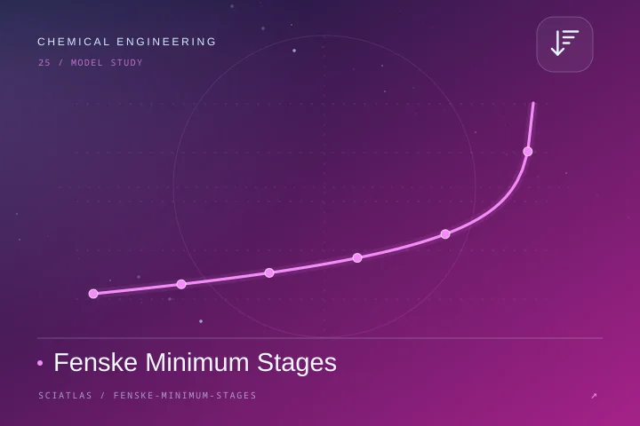
Fenske Minimum Stages
Nmin=ln[(xD/(1−xD))((1−xB)/xB)]/lnα: Calculate the Fensk minimum theoretical level based on the input, and provide local sensitivity curves and data export.
Total reflux binary approximation, including equilibrium reboiler; results are not rounded up to show continuous values.
Reactor Space Time
τ=V/Q: Calculate the average residence time of the reactor based on the input, and provide local sensitivity curves and data export.
Constant density steady flow; not equal to the actual residence time of all particles.

First Order Damkohler
Da=kτ: Calculate the Damköhler number of the first-order reaction based on the input, and provide local sensitivity curves and data export.
First-order isothermal kinetics, flow model to be specified separately.
First Order CSTR Conversion
X=kτ/(1+kτ): Calculate the first-level CSTR conversion rate based on the input, and provide local sensitivity curves and data export.
Ideal complete mixing, constant temperature, constant density, first-order irreversible reaction.
First Order PFR Conversion
X=1−exp(−kτ): Calculate the first-level PFR conversion rate based on the input, and provide local sensitivity curves and data export.
Ideal plug flow, constant temperature and constant density first-order irreversible reaction.
Langmuir Adsorption
q=qmax KC/(1+KC): Calculate the Langmuir adsorption isotherm based on the input, and provide local sensitivity curves and data export.
Uniform independent sites, monolayer, constant temperature equilibrium.
Understand the method and then start calculating
Tools in this field provide runnable examples, model conditions and method descriptions. Please select a model that meets the experimental conditions and retain parameter and version information.
Connect knowledge with each other
Related disciplines and tools In the initial calculation of
Mechanical Engineering ↗fluid equipment and loads
Microbiology ↗bioreactor and mass transfer
Pharmacokinetics ↗room model and material conservation