Earth & Geophysics
From questions to insights, 30online scientific tool. No registration required, free calculation and export.

Well Log Studio
allows depth, formation and logging curves to be clearly displayed on the same picture.
CSV numerical curve; depth downward; each curve is displayed in separate tracks. Lithology can be represented by an additional numeric column. The first row of the
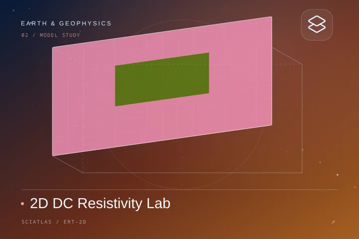
2D DC Resistivity Lab
fits a parameterized subsurface resistivity model from DC potential observations.
2D finite volume forward modeling; fixes the anomaly body geometry and only inverts the two resistivities of the background and the anomaly body. The closed sides and bottom surface have zero potential, which belongs to the finite box model; an example of synthetic verification using empty data.

3D DC Resistivity Lab
fits a parameterized subsurface resistivity model from DC potential observations.
3D finite volume forward modeling; fixed anomaly body geometry, only inverts the two resistivities of background and anomaly body. The closed sides and bottom surface have zero potential, which belongs to the finite box model; an example of synthetic verification using empty data.
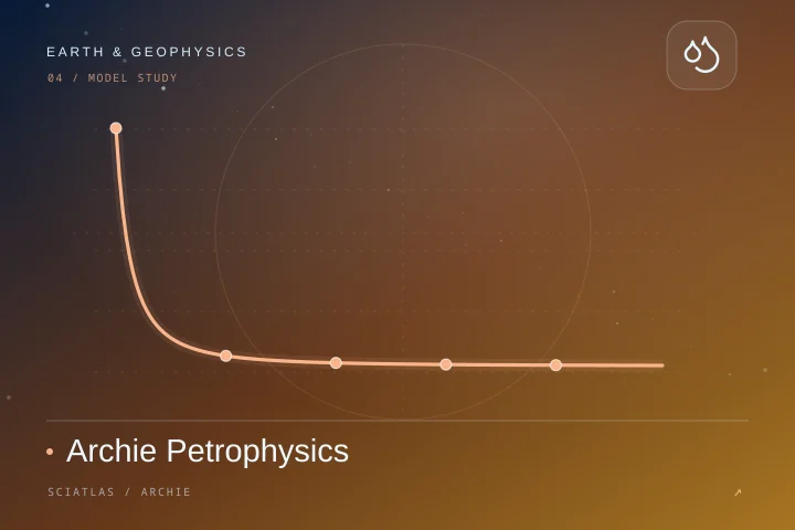
Archie Petrophysics
uses Archie relationship to analyze porosity, water saturation and formation resistivity.
clean clay-free rock empirical model, parameters must be calibrated according to rock samples.

Darcy Flow
calculates seepage volume, Darcy flux, and pore flow velocity from hydraulic gradients.
Saturated, laminar flow, homogeneous one-dimensional porous medium.
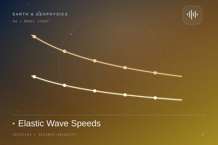
Elastic Wave Speeds
calculates P/S wave speed, wave impedance and Poisson's ratio.
Uniform isotropic linear elastic medium.
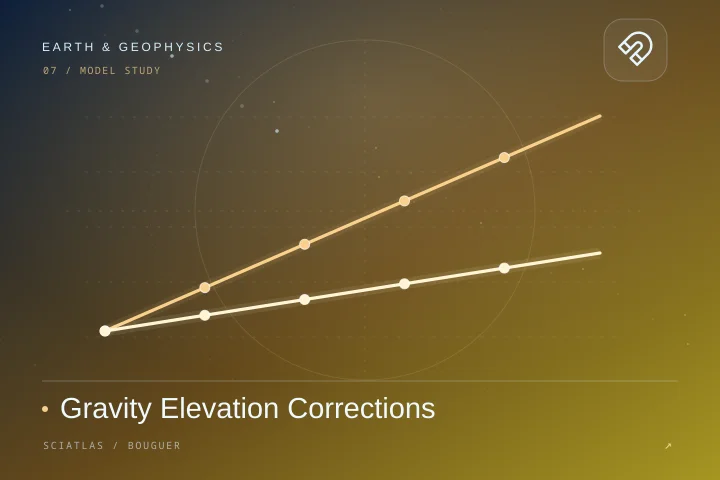
Gravity Elevation Corrections
computes the plate Bouguer term and first-order free air correction.
Infinite horizontal plate, first-order elevation approximation, excluding terrain and latitude corrections.
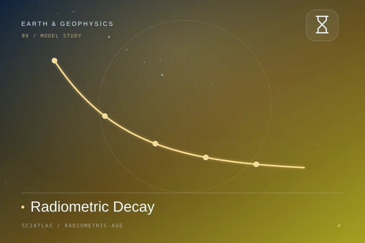
Radiometric Decay
estimates the age of a closed system from the remaining proportion of the parent and the half-life.
Single nuclide, initial parent is known, no migration in or out.

Infinite Slope
estimates the anti-slip safety factor of a uniform shallow sliding surface.
Infinite slope static model, parallel slope sliding; not engineering design certification.
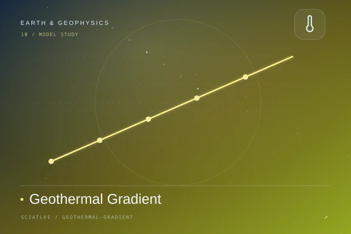
Geothermal Gradient
calculates linear temperature profiles for formations with constant thermal conductivity.
One-dimensional steady state, no internal heat source and groundwater convection.
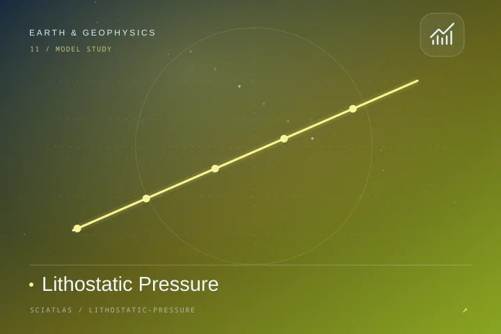
Lithostatic Pressure
P=ρgz: Calculate lithostatic pressure based on input, and provide local sensitivity curves and data export.
Uniform density vertical rock column; does not contain additional structural stress.
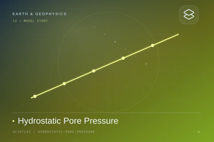
Hydrostatic Pore Pressure
u=ρwgz: Calculate hydrostatic pore pressure based on input, and provide local sensitivity curves and data export.
connects to the stationary water column; does not include overpressure and capillary pressure.
Terzaghi Effective Stress
σ′=σ−u: Calculate Terzaghi effective stress based on input, and provide local sensitivity curves and data export.
One-dimensional stress scalar of saturated soil; negative values indicate that the set parameters may cause splaying or instability.
Normal Reflection Coefficient
R=(ρ₂v₂−ρ₁v₁)/(ρ₂v₂+ρ₁v₁): Calculate the normal reflection coefficient based on the input, and provide local sensitivity curves and data export.
Plane interface, normal incidence acoustic approximation; ignores shear converted waves.
Seismic Critical Angle
θc=asin(v₁/v₂): Calculate the critical angle of seismic refraction based on the input, and provide local sensitivity curves and data export.
requires that the wave speed of the lower layer is not less than that of the upper layer, calculated based on the flat horizontal interface.
Two-way Travel-time Depth
z=vt/2: Calculate the two-way travel time depth based on the input, and provide local sensitivity curves and data export.
Vertical propagation, known average velocity; oblique incidence and velocity gradient need to be processed independently.
GPR Depth
z=ct/(2√εr): Calculate ground penetrating radar depth based on input, provide local sensitivity curve and data export.
Low-loss non-magnetic homogeneous medium; the dielectric constant should be calibrated by actual measurement.
EM Skin Depth
δ=√[ρ/(πfμ₀)]: Calculate the electromagnetic skin depth based on the input, and provide local sensitivity curves and data export.
Good conductor, non-magnetic uniform half space, ignore displacement current.
Wenner Apparent Resistivity
ρa=2πaΔV/I: Calculate the Wenner apparent resistivity based on the input, and provide local sensitivity curves and data export.
Equally spaced surface Wenner array; the result is the apparent resistivity, not the inversion of the true formation value.
Aquifer Transmissivity
T=Kb: Calculate the aquifer hydraulic conductivity based on the input, and provide local sensitivity curves and data export.
Homogeneous aquifer; heterogeneous profiles need to be integrated along the thickness.
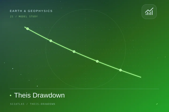
Theis Drawdown
s=Q E₁(r²S/4Tt)/(4πT): Calculate the Theis depth drop based on the input, and provide local sensitivity curves and data export.
Infinitely confined aquifer, completely penetrating well, constant pumping; does not include boundaries and well losses.

Stokes Settling
v=(ρp−ρf)gd²/(18μ): Calculates particle Stokes settlement based on input, providing local sensitivity curves and data export.
Isolated spherical particles, low Reynolds number; compulsory check |Re|<0.1.
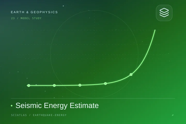
Seismic Energy Estimate
log₁₀E=1.5Mw+4.8: Calculate the earthquake energy magnitude based on the input, and provide local sensitivity curves and data export.
Empirical radiation energy relationship is only used for magnitude estimation rather than precise event-by-event inversion.

Seismic Moment
M₀=μAD: Calculate the seismic scalar moment based on the input, and provide local sensitivity curves and data export.
Finite fault approximation for uniform shear modulus and plane-averaged slip.

Moment Magnitude
Mw=(2/3)(log₁₀M₀−9.1): Calculate the seismic moment torque magnitude based on the input, and provide local sensitivity curves and data export.
adopts SI seismic moment constant 9.1; there are slight differences in calibration based on different experiences.

Mohr Coulomb Strength
τ=c+σ′tanφ: Calculate the molar Coulomb shear strength based on the input, and provide local sensitivity curves and data export.
Linear intensity envelope, excluding strain softening or unsaturated suction.

Rankine Active Coefficient
Ka=(1−sinφ)/(1+sinφ): Calculate the Rankine active earth pressure coefficient based on the input, and provide local sensitivity curves and data export.
Horizontal fill, smooth vertical walls, no cohesion; does not include additional earthquake loads.

Rankine Passive Coefficient
Kp=(1+sinφ)/(1−sinφ): Calculate the Rankine passive earth pressure coefficient based on the input, and provide local sensitivity curves and data export.
Assuming horizontal fill and smooth vertical wall, the passive state requires sufficient displacement.

Geothermal Heat Flux
q=k∇T: Calculate geothermal conduction heat flow based on input, and provide local sensitivity curves and data export.
calculates the magnitude of upward heat flow based on the temperature gradient in the direction of increasing depth, excluding groundwater convection.

Stable Isotope Delta
δ=1000(R/Rstd−1): Calculate the stable isotope δ value based on the input, and provide local sensitivity curves and data export.
The sample and standard must use the same weight and light isotope ratio definitions.
Understand the method and then start calculating
Tools in this field provide runnable examples, model conditions and method descriptions. Please select a model that meets the experimental conditions and retain parameter and version information.
Connect knowledge with each other
Related disciplines and tools In the initial calculation of
Agronomy & Climate ↗Soil hydrology, groundwater and irrigation
Materials & Crystals ↗Mineral crystals, pores and media properties
Mathematics ↗Measurement Inversion and Uncertainty