Quantum Science
From questions to insights, 30online scientific tool. No registration required, free calculation and export.
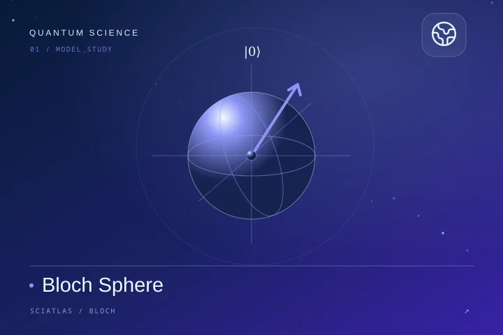
Bloch Sphere
Rotate state vectors and understand the phase and measurement of single qubits.
Pure state single bit; spherical coordinates θ/φ initialized, specified gates applied in sequence.
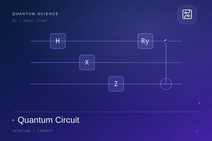
Quantum Circuit
combines quantum gates to view amplitude, probability and reproducible measurement samples.
1–8 bit status vector; H/X/Y/Z/S/T, RX/RY/RZ, CX; q0 is the least significant bit. OpenQASM 2.0 exports are supported for the subset listed.

Density Matrix
View Bell states, mixed noise and reduced quantum states.
Mixture of two-bit Bell state and maximum mixed state ρ=(1−p)|Φ+ ⟨Φ+|+pI/4; indicators are purity, reduced entropy and negativity.
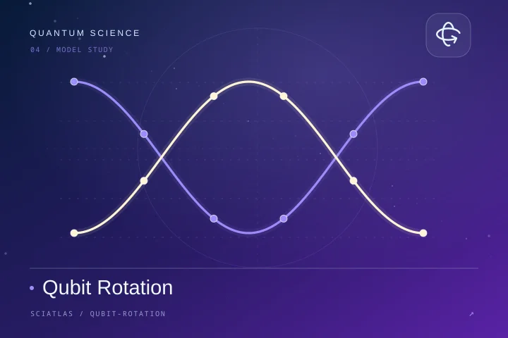
Qubit Rotation
Calculates the amplitude and measurement probability of Ry(θ)|0 .
Ideal single bit, no noise; base order is |0 , |1 .
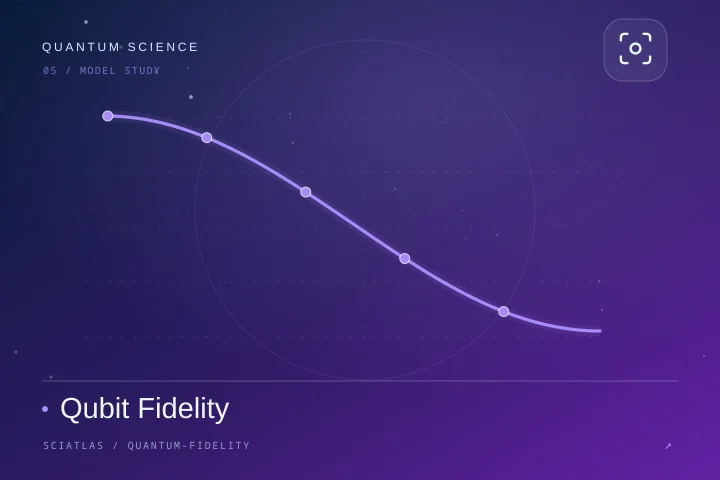
Qubit Fidelity
Compares the overlap and distinguishability of two Bloch sphere pure states.
Pure state fidelity adopts the square convention F=|⟨ψ|φ |².
Bell CHSH Correlations
computes the CHSH combination of spin singlets in the plane measurement direction.
Ideal spin singlet E(a,b)=−cos(a−b), the angle is the Bloch measurement axis angle; not the physical angle of the photon polarizer.
Particle in a Box
calculates the energy levels and selected state probability density of a one-dimensional infinitely deep potential well.
Non-relativistic particles, infinite potential barriers, and zero potential energy in the well; the particle mass is input as a multiple of the electron mass.
Quantum Harmonic Oscillator
Calculates equally spaced energy levels, zero point energy and average occupancy number of thermal excitations.
Ideal one-dimensional resonator, Bose thermal balance; does not contain anharmonicity.

Rectangular Barrier Tunneling
Calculates transmission probability and width effects below the barrier energy.
One-dimensional, equal-mass, rectangular potential barrier, 0<E<V0; coherent stationary scattering.

Gaussian Wavepacket
plots the normalized position density and computes the minimum uncertain momentum broadening.
is the minimum uncertain Gaussian pure state, Δx is the position standard deviation, excluding propagation and external potential.

De Broglie Wavelength
λ=h/p: Calculate the de Broglie wavelength based on the input, and provide local sensitivity curves and data export.
uses the definition of momentum; the relativistic range needs to be considered when determining momentum from velocity.
Electron Wavelength
λ=h/√(2meV): Calculate the electron acceleration voltage wavelength according to the input, and provide local sensitivity curves and data export.
Non-relativistic electrons accelerate from rest, high voltage requires relativistic correction.
Photon Frequency Energy
E=hf: Calculate photon frequency energy according to input, provide local sensitivity curve and data export.
Free photon frequency to energy conversion.
Photon Wavelength Energy
E=hc/λ: Calculate the photon wavelength energy based on the input, and provide local sensitivity curves and data export.
Vacuum wavelength, do not mix wavelengths in the medium.

Momentum Uncertainty Bound
Δp≥ℏ/(2Δx): Calculate the position momentum uncertainty lower bound based on the input, and provide local sensitivity curves and data export.
is the lower bound of the standard deviation uncertainty relationship, which is not equal to the instrument error formula.
Lifetime Energy Width Scale
ΔE≈ℏ/(2τ): Calculate the lifetime energy width magnitude based on the input, and provide local sensitivity curves and data export.
time energy magnitude convention, line width definition and specific decay model may have factor differences.

Hydrogenic Bohr Radius
rn=a₀n²/Z: Calculate the hydrogen-like Bohr orbital scale based on the input, and provide local sensitivity curves and data export.
is the scale of the non-relativistic single-electron Bohr model, not the real electron trajectory.

Hydrogenic Energy Level
En=−13.605693 Z²/n²: Calculate the hydrogen sample energy level based on the input, and provide local sensitivity curves and data export.
Infinitely heavy nuclear single electron non-relativistic approximation; relativistic and finite nuclear corrections are required at high Z.
Rydberg Transition Wavelength
1/λ=R∞ Z²(1/nf²−1/ni²): Calculate the hydrogen sample transition wavelength based on the input, and provide local sensitivity curves and data export.
Hydrogen-like atomic emission, ignoring reduced mass and fine structure.
Compton Wavelength Shift
Δλ=h(1−cosθ)/(mec): Calculate the Compton wavelength shift based on the input, and provide local sensitivity curves and data export.
Initial stationary free electron scattering.
Photoelectric Kinetic Energy
Kmax=max(hc/λ−Φ,0): Calculate the maximum kinetic energy of photoelectrons based on the input, and provide local sensitivity curves and data export.
Single photon surface photoelectric effect; zero indicates insufficient escape or threshold and does not describe multiphoton processes.
Resonant Rabi Probability
P=sin²(Ωt/2): Calculate the resonance Rabi transition probability based on the input, and provide local sensitivity curves and data export.
No detuning, no decoherence, ideal two-level drive.
Detuned Rabi Probability
P=Ω²/(Ω²+Δ²) sin²(√(Ω²+Δ²)t/2): Calculate the detuned Rabi transition based on the input, and provide local sensitivity curves and data export.
Spin wave approximation, fixed amplitude drive and noiseless two-level system.
Qubit T1 Relaxation
Pe=Pe₀exp(−t/T1): Calculate the qubit T1 attenuation based on the input, and provide local sensitivity curves and data export.
Zero-temperature Markov amplitude decay, no thermal excitation.
Qubit T2 Coherence
c=c₀exp(−t/T2): Calculate quantum coherent T2 attenuation based on input, provide local sensitivity curves and data export.
exponential coherence envelope; consistency with specified T1 is not independently guaranteed.

Bloch Vector Purity
Trρ²=(1+r²)/2: Calculate Bloch vector purity based on input, provide local sensitivity curve and data export.
single qubit density matrix, 0≤r≤1.
Qubit Von Neumann Entropy
S=H₂[(1+r)/2]: Calculate single-bit von Neumann entropy based on input, provide local sensitivity curves and data export.
Single-bit spectral entropy, the pure state is zero and the maximum mixed state is one.
Spin Thermal Polarization
P=tanh(ΔE/(2kBT)): Calculate the spin thermal equilibrium polarization based on the input, and provide local sensitivity curves and data export.
non-degenerate two-level thermal equilibrium model.
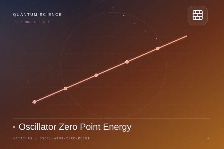
Oscillator Zero Point Energy
E₀=hf/2: Calculate the zero-point energy of the resonator based on the input, and provide local sensitivity curves and data export.
Ground state energy of one-dimensional ideal quantum oscillator.
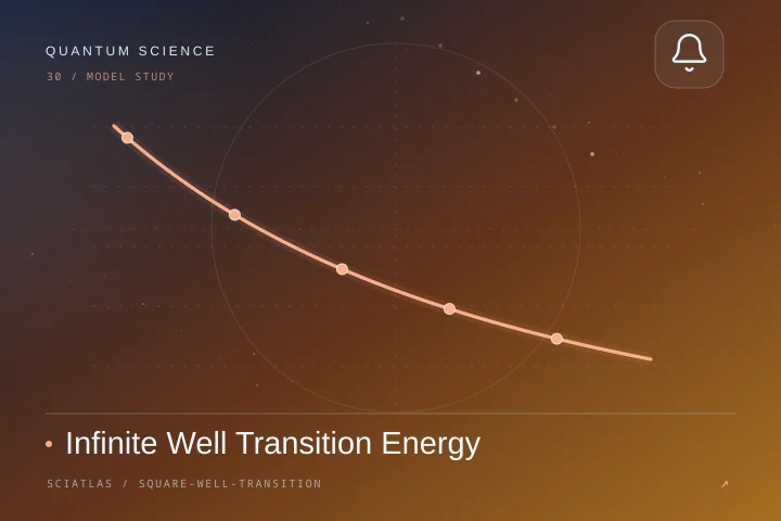
Infinite Well Transition Energy
ΔE=h²(n₂²−n₁²)/(8mL²): Calculate the infinite deep well transition energy based on the input, and provide local sensitivity curves and data export.
One-dimensional infinite deep well; the positive value is the absorption energy difference and does not include selection rule judgment.
Understand the method and then start calculating
Tools in this field provide runnable examples, model conditions and method descriptions. Please select a model that meets the experimental conditions and retain parameter and version information.
Connect knowledge with each other
Related disciplines and tools In the initial calculation of
Materials & Crystals ↗Quantum Devices and Electron Microscopy The
Cryptography ↗Quantum Algorithm and Key System
Mathematics ↗Complex vectors, operators and probability